Broadcasting example program in python

 The term broadcasting refers to the ability of NumPy to treat arrays of different shapes during arithmetic operations. Arithmetic operations on arrays are usually done on corresponding elements. If two arrays are of exactly the same shape, then these operations are smoothly performed.

If the dimensions of two arrays are dissimilar, element-to-element operations are not possible. However, operations on arrays of non-similar shapes is still possible in NumPy, because of the broadcasting capability. The smaller array is broadcast to the size of the larger array so that they have compatible shapes.

Broadcasting is possible if the following rules are satisfied −

1.     Array with smaller ndim than the other is prepended with '1' in its shape.
2.     Size in each dimension of the output shape is maximum of the input sizes in that dimension.
3.     An input can be used in calculation, if its size in a particular dimension matches the output size or its value is exactly 1.
4.     If an input has a dimension size of 1, the first data entry in that dimension is used for all calculations along that dimension.
   

A set of arrays is said to be broadcastable if the above rules produce a valid result and one of the following is true −

1.     Arrays have exactly the same shape.
2.     Arrays have the same number of dimensions and the length of each dimension is either a common length or 1.
3.     Array having too few dimensions can have its shape prepended with a dimension of length 1, so that the above stated property is true.

The following program shows an example of broadcasting. 

import numpy as np 
a = np.array([[0.0,0.0,0.0],[10.0,10.0,10.0],[20.0,20.0,20.0],[30.0,30.0,30.0]]) 
b = np.array([1.0,2.0,3.0])  
   
print('First array:')
print(a) 
print('\n')  
   
print('Second array:') 
print(b)
print('\n')  
   
print('First Array + Second Array') 
print(a + b)

The Output is as follow

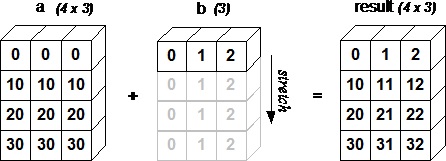
First array:
[[ 0.  0.  0.]
 [10. 10. 10.]
 [20. 20. 20.]
 [30. 30. 30.]]


Second array:
[1. 2. 3.]


First Array + Second Array
[[ 1.  2.  3.]
 [11. 12. 13.]
 [21. 22. 23.]
 [31. 32. 33.]]

The following figure demonstrates how array b is broadcast to become compatible with a.

 Reference:www.tutorialspoint.com