Mean Removal data pre-processing technique on sample data machine learning

 Mean Removal in Machine Learning is a type of data pre-processing technique which is used to remove a mean from every feature so that it could center on zero. It also helps in removing bias from the feature.

In the real world, we usually have to deal with a lot of raw data. This raw data is not readily ingestible by machine learning algorithms. To prepare data for machine learning, we have to preprocess it before we feed it into various algorithms. This is an intensive process that takes plenty of time, almost 80 percent of the entire data analysis process, in some scenarios. However, it is vital for the rest of the data analysis workflow, so it is necessary to learn the best practices of these techniques. Before sending our data to any machine learning algorithm, we need to cross check the quality and accuracy of the data. If we are unable to reach the data stored in Python correctly, or if we can't switch from raw data to something that can be analyzed, we cannot go ahead. Data can be preprocessed in many ways—standardization, scaling, normalization, binarization, and one-hot encoding are some examples of preprocessing techniques. 

Standardization of datasets is a common requirement for many machine learning estimators implemented in scikit-learn; they might behave badly if the individual features do not more or less look like standard normally distributed data: Gaussian with zero mean and unit variance.

In practice we often ignore the shape of the distribution and just transform the data to center it by removing the mean value of each feature, then scale it by dividing non-constant features by their standard deviation.

For instance, many elements used in the objective function of a learning algorithm (such as the RBF kernel of Support Vector Machines or the l1 and l2 regularizers of linear models) assume that all features are centered around zero and have variance in the same order. If a feature has a variance that is orders of magnitude larger than others, it might dominate the objective function and make the estimator unable to learn from other features correctly as expected.

Example

from sklearn import preprocessing
import numpy as np
X_train = np.array([[ 1., -1.,  2.],
                    [ 2.,  0.,  0.],
                    [ 0.,  1., -1.]])
scaler = preprocessing.StandardScaler().fit(X_train)
scaler


scaler.mean_


scaler.scale_


X_scaled = scaler.transform(X_train)
X_scaled

Output

array([[ 0.        , -1.22474487,  1.33630621],
       [ 1.22474487,  0.        , -0.26726124],
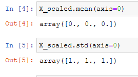
       [-1.22474487,  1.22474487, -1.06904497]])

 Scaled data has zero mean and unit variance:

You can see that the mean is almost 0 and the standard deviation is 1.