Probability Distributions in Data Science

What Is Probability?

Probability denotes the possibility of something happening. It is a mathematical concept that predicts how likely events are to occur. The probability values are expressed between 0 and 1. The definition of probability is the degree to which something is likely to occur. This fundamental theory of probability is also applied to probability distributions.

What Are Probability Distributions?

A probability distribution is a statistical function that describes all the possible values and probabilities for a random variable within a given range. This range will be bound by the minimum and maximum possible values, but where the possible value would be plotted on the probability distribution will be determined by a number of factors. The mean (average), standard deviation, skewness, and kurtosis of the distribution are among these factors.

Types of Probability Distribution

The probability distribution is divided into two parts:

1. Discrete Probability Distributions
2. Continuous Probability Distributions

Discrete Probability Distribution

A discrete distribution describes the probability of occurrence of each value of a discrete random variable. The number of spoiled apples out of 6 in your refrigerator can be an example of a discrete probability distribution.

Each possible value of the discrete random variable can be associated with a non-zero probability in a discrete probability distribution.

Let's discuss some significant probability distribution functions.

1. Binomial Distribution

The binomial distribution is a discrete distribution with a finite number of possibilities. When observing a series of what are known as Bernoulli trials, the binomial distribution emerges. A Bernoulli trial is a scientific experiment with only two outcomes: success or failure.

Consider a random experiment in which you toss a biased coin six times with a 0.4 chance of getting head. If 'getting a head' is considered a ‘success’, the binomial distribution will show the probability of r successes for each value of r.

The binomial random variable represents the number of successes (r) in n consecutive independent Bernoulli trials.

2. Bernoulli's Distribution

The Bernoulli distribution is a variant of the Binomial distribution in which only one experiment is conducted, resulting in a single observation. As a result, the Bernoulli distribution describes events that have exactly two outcomes.

Here’s a Python Code to show Bernoulli distribution:

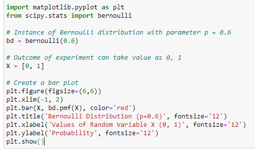
The Bernoulli random variable's expected value is p, which is also known as the Bernoulli distribution's parameter.

The experiment's outcome can be a value of 0 or 1. Bernoulli random variables can have values of 0 or 1.

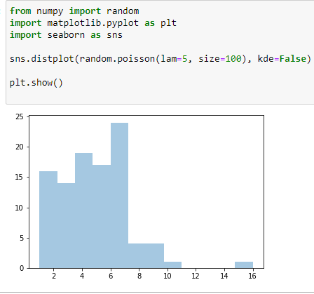
3. Poisson Distribution

A Poisson distribution is a probability distribution used in statistics to show how many times an event is likely to happen over a given period of time. To put it another way, it's a count distribution. Poisson distributions are frequently used to comprehend independent events at a constant rate over a given time interval. Siméon Denis Poisson, a French mathematician, was the inspiration for the name.

The Python code below shows a simple example of Poisson distribution. 

It has two parameters:

1. Lam: Known number of occurrences
2. Size: The shape of the returned array

The below-given Python code generates the 1x100 distribution for occurrence 5.

Continuous Probability Distributions

A continuous distribution describes the probabilities of a continuous random variable's possible values. A continuous random variable has an infinite and uncountable set of possible values (known as the range). The mapping of time can be considered as an example of the continuous probability distribution. It can be from 1 second to 1 billion seconds, and so on.

The area under the curve of a continuous random variable's PDF is used to calculate its probability. As a result, only value ranges can have a non-zero probability. A continuous random variable's probability of equaling some value is always zero.

Now, look at some varieties of the continuous probability distribution.

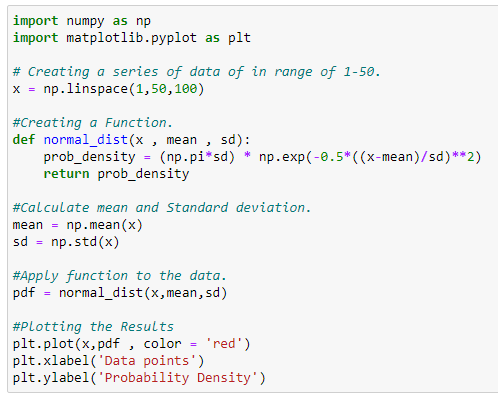
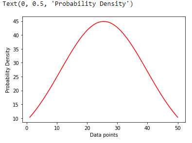
4. Normal Distribution

Normal Distribution is one of the most basic continuous distribution types. Gaussian distribution is another name for it. Around its mean value, this probability distribution is symmetrical. It also demonstrates that data close to the mean occurs more frequently than data far from it. Here, the mean is 0, and the variance is a finite value.

In the example, you generated 100 random variables ranging from 1 to 50. After that, you created a function to define the normal distribution formula to calculate the probability density function. Then, you have plotted the data points and probability density function against X-axis and Y-axis, respectively.

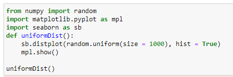
Continuous Uniform Distribution

In continuous uniform distribution, all outcomes are equally possible. Each variable has the same chance of being hit as a result. Random variables are spaced evenly in this symmetric probabilistic distribution, with a 1/ (b-a) probability.

The below Python code is a simple example of continuous distribution taking 1000 samples of random variables.

 Reference: https://www.simplilearn.com